Chapters
Statistics

Statistics Glossary
Chapters
Table of Contents
1) Basics
Statistics: Statistics is the discipline that concerns the collection, organization, analysis, interpretation, and presentation of data
Observation: (interchangably used with value) An observation is the value, at a particular period, of a particular variable
Variable: A variable is a storage of observations, which can vary w.r.t. to time or event
Descriptive Statistics: Methods used to summarize or describe our observations
Inferential Statistics: Using those summarizations for making estimates or predictions, i.e. inferences, about a situation that has not yet been investigated
Population: All the case or situations, that the statisticians want their inferences

Sample: A subset of the population

Random: Each member of the population having equal chance of getting selected for a sample
Stratified Random Sample: Each strata (i.e. individual class) having equivalent
representation in the sample
i.e. if a bag has population of 100 balls, i.e. 52 red, 24 green and 24 blue, then aafter
performing Stratified sampling for 50 balls out of the bag, i.e. (50% of population) will have
26 red, 12 green & 12 blue balls. Choice of balls would be random, but count of balls would be a
representation of their strata in population
Describing A Sample
Category: Category is a class or division of people or things regarded as having particular shared characteristics, e.g. the Red Balls category share similar characteristics of being Red in color
Category Variables: Any varibale, that involves putting individuals into categories
Quantitative variables: Variables which carries data that is either measure of values or counts, and are expressed as numbers, e.g. Continous(length of a mobile screen) & Discrete(number of mobiles)
Qualitative variables: Qualitative variables carries data that is measure of 'types' and may be represented by a name, symbol, or a number code, e.g. Nominal & Ordinal variables
Nominal Variables: Nominalis is latin for name, thus, nominal variables represents
differnt names a varibale may take.
e.g. Name, Adress, Description, Product_Type, etc.
Ordinal Variable: A variable which helps us to disctinctly arrange sample members into in
an orderly fashion
e.g. Grades, Rating, etc.
Discrete Variable: A variable that represents a value, which countable, i.e. one in which the possible values are clearly separated, e.g. 1 Train, 2 Trucks, 3 Apples, 4 Niqqah, 5 Occeans, etc.
Continous Variable: A vriable that represents a value, which is not countable as they are not clearly sperable, but measurable, e.g. while measuring length with a measuring tape, the length could be 12.3cm or 12.324cm or 12.324123456cm all could represent 1 single value, depending upon the precision of measuring instrument, thus not clearly separable from each other, unlike 1-measuring tape, 2-measuring tape, and so on
Type Conversion: Quantitative data can be converted into Qualitative data, i.e. converting marks to Grades, however, this leads to Information Loss, as converted data can't be brought back to its precise past value
Data Summary
Table: A table is
a set of facts or figures, systematically displayed in columns
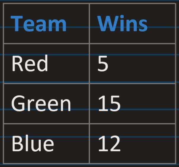
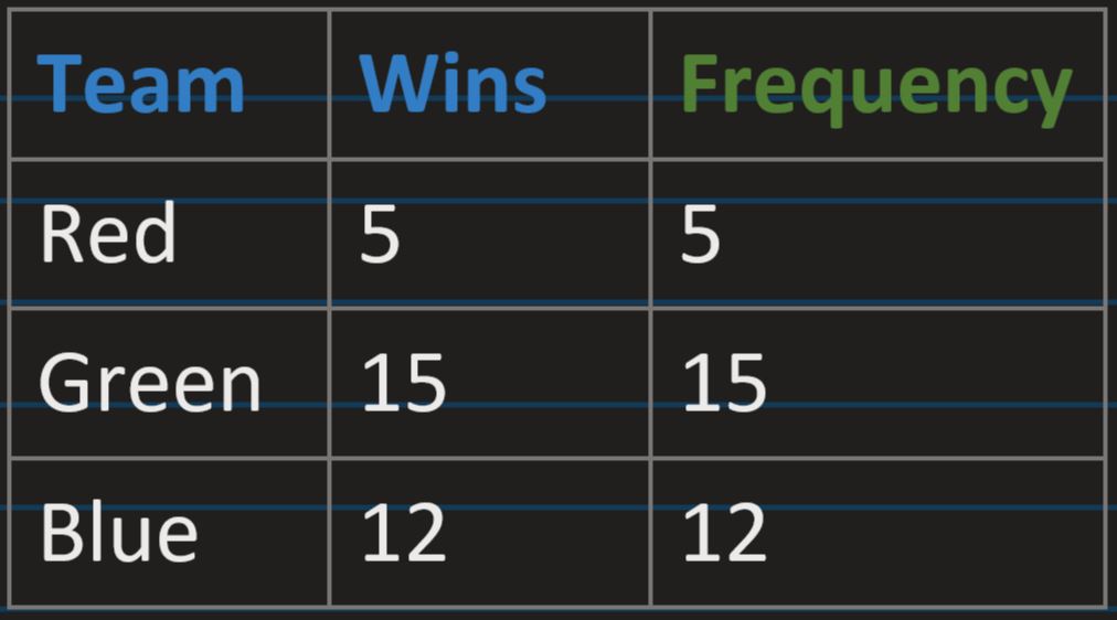
Frequency Table: Representation of data in the form of showing frequency, for each
category
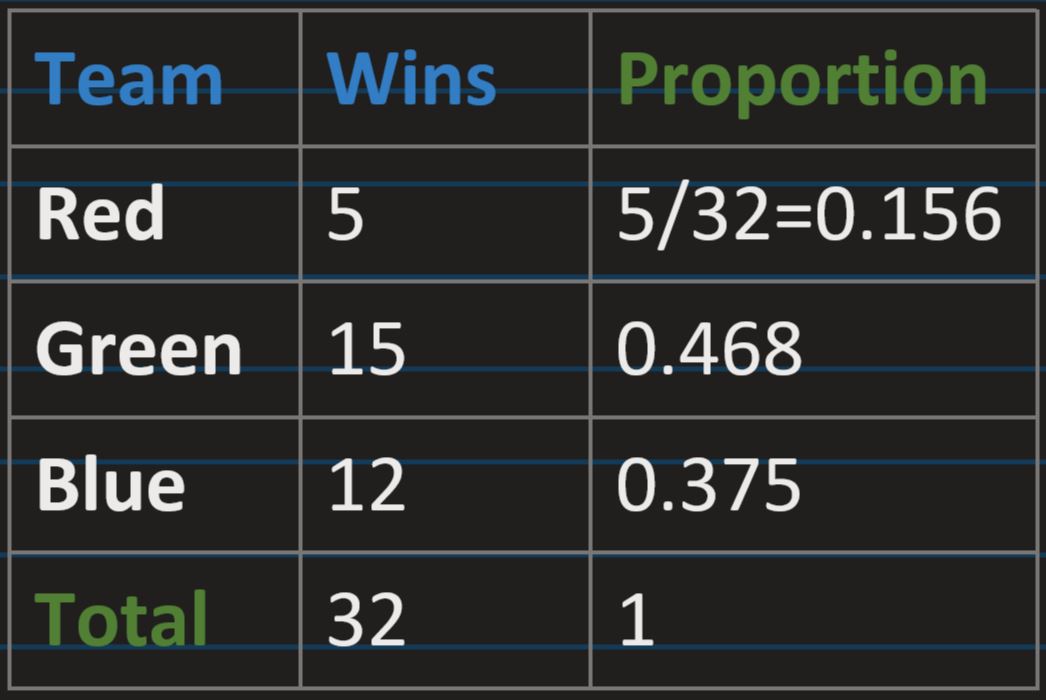
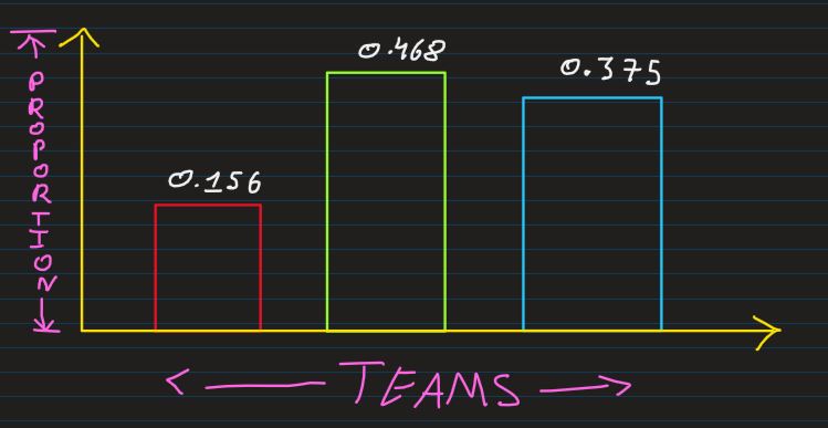
Proportion: a share in comparative relation to a whole
Block Diagram: The proportion table can be graphically visualized using a graph
representing
categories and proportion in X & Y axis, respectively
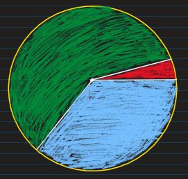
Pie Chart: A non-linear form to represent the same information is Pie Chart
Distribution: Lets considere few observations. Below given is the observation of number
of student present in a class, where each cell represent a unique class
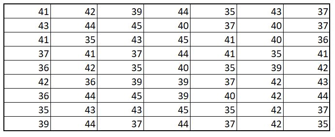
Data in this format is not easy to digest and defintely not the best we can present in. A sinple
enhancement to this would be, to arrange them in an order, i.e. Increasing or Decreasing
order. Now,
each of the column is sorted
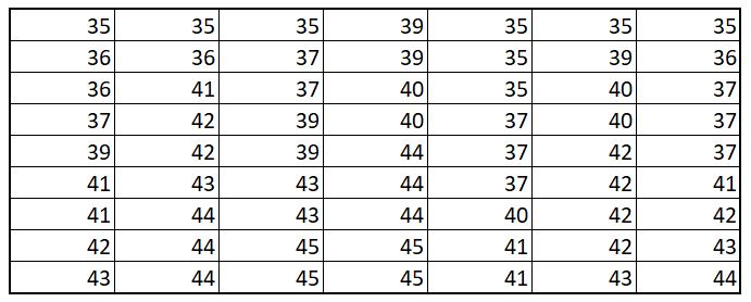 What we created above is called a Distribution, i.e. an orderly arranged quantitative
variable
What we created above is called a Distribution, i.e. an orderly arranged quantitative
variable
Range: The differnce between the maximum and minimum value in a distribution is called
the
distribution's range, e.g. in the below example, the range of the distribution is 60-21, i.e. 39
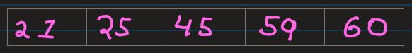
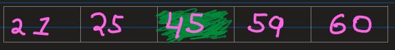
Median: (latin for middle)For a distribution, lets say 21, 25, 45, 59 & 60, the
value located
at the middle is its median. Thus, for the given distribution, the median value is 45
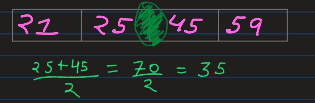
And since we can't have a "1-midpoint" in case of even number of observations,
so instead, the values which divide the distribution in equal left & right halves
(25&45 divides this even distribution in 2 equal halved), we would take the mid-distance
between those values as our median value
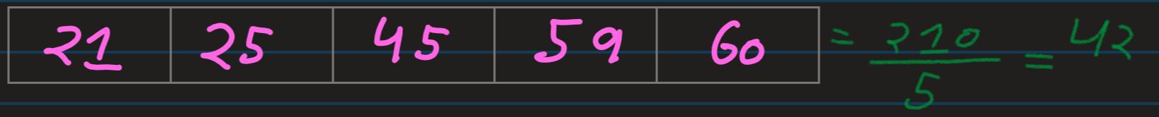
Arithmetic Mean: Although Median is a good representative value of a distribution, but
far more
quoted one is Average. Almost every time someone mentions Average, they are talking
about Arithmetic Mean, not the other kind of
means.
Arithmetic Mean is, addition of all the values in a distribution, and dividing the sum with the
number of
observations
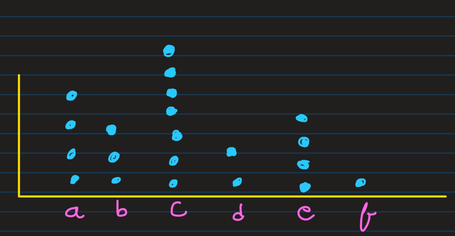
Dot Diagram: Distribution (orderly arranged) is better to digest as
compared to raw form, this can still be further optimized, by using graphical illustraion
instead of
directly crunching or looking at each value in the observation
E.g. lets look at the below recorded values
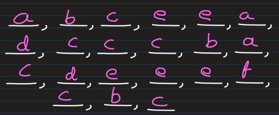
A much optimized way of looking at it, instead of reading each and every occurence of values
would be
Dot Diragram, i.e. pictorial frequency distribution table
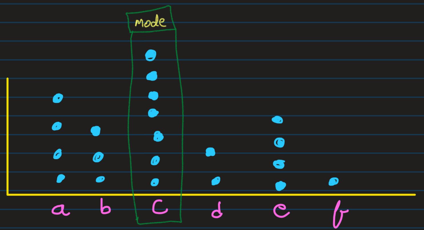
Mode: In our dot diagram, the value with greatest frequency is called as Mode of the
distribution
In the above given distribution, it is found that 37 is the Mode of the distribution
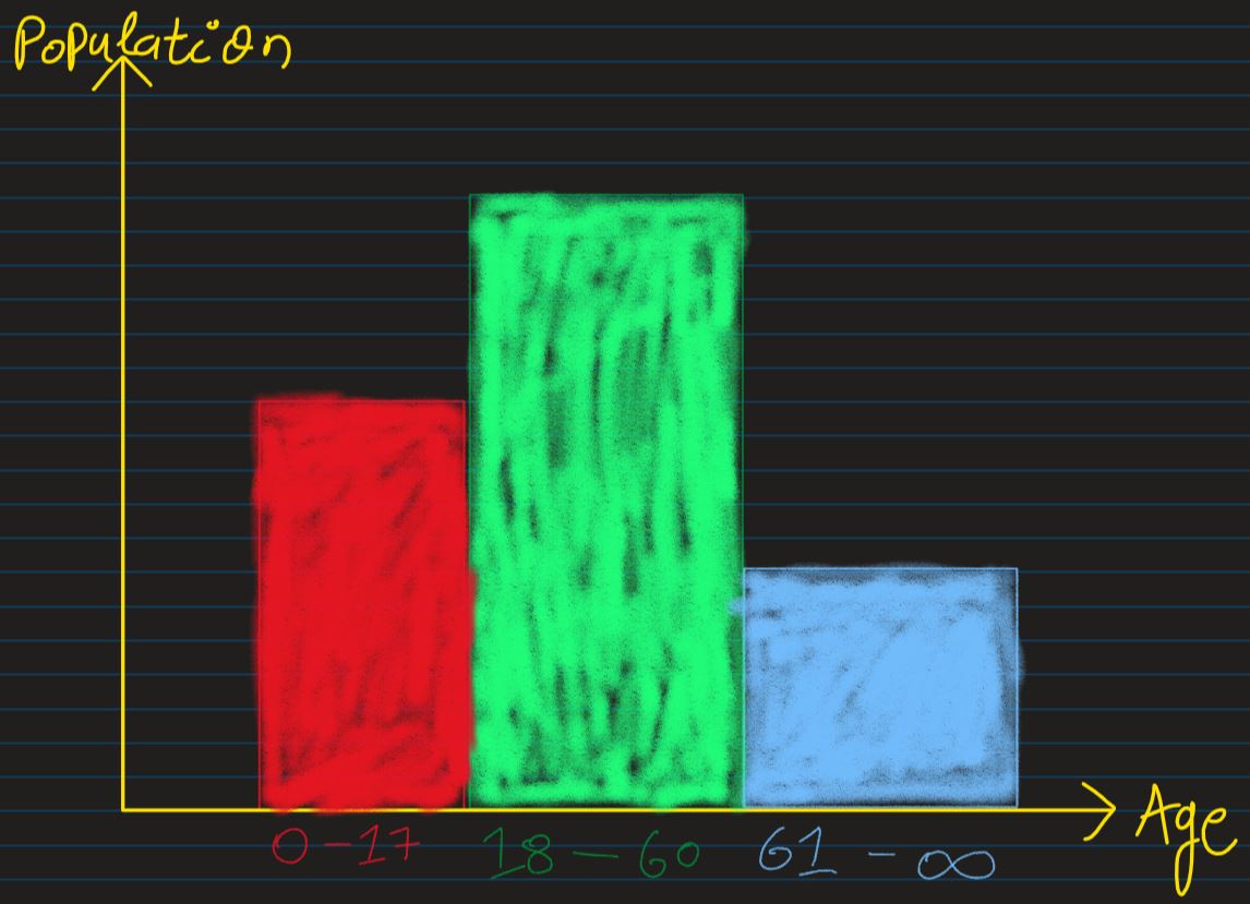
Histogram: Another way of representing frequency distribution, specially in situation
where unique
observations are too large, is to group the observations in buckets, i.e. via type
conversion of
quantitative data into categoprical buckets, and then plot its block diagram
Central Tendency: It is crucial to have some ways to quanitfy the distribution, and 2 of
them are
central tendency and variability
Central Tendency of the distribution is, the distribution's tendency to pile up, arround a
particular value,
instead of spreading out evenly acorss a range. E.g. Mean, Median & Mode
Dispersion
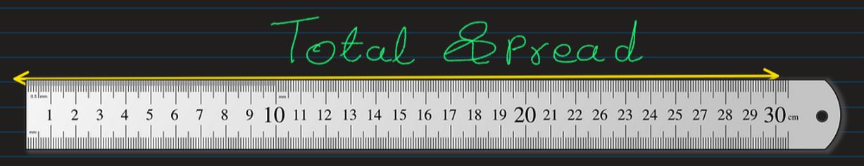
Lets taalk a bit about dispersion too. Dispersion is about spread of data. Remeber median? That
is going to help us in measuring dispersion
Lets assume the below given images tells about the total
spread of the
distribution
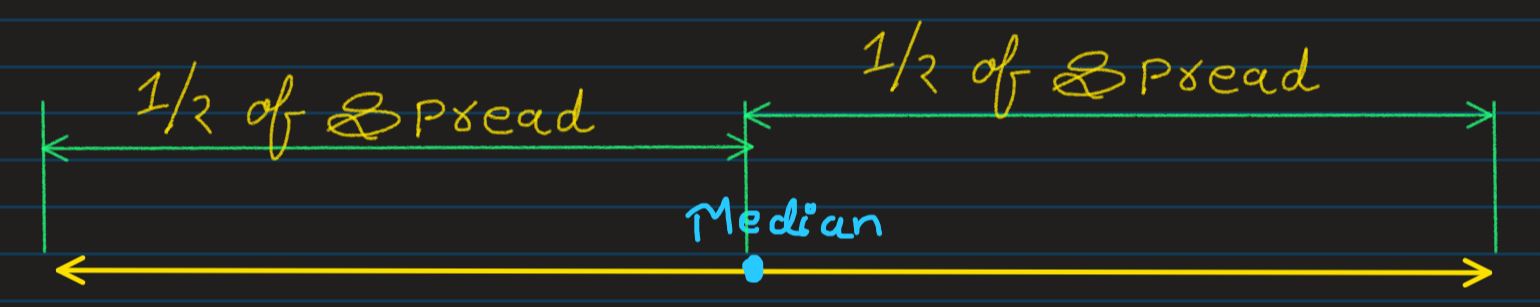
 Lets plot a median in this spread of data
 Now divide the left region from median, into 2 equal halves, and mark the point which divides
the left portion into
2 equal halves as Q1. And similarly, do the same for right region from the median, and
mark it as Q3
Now divide the left region from median, into 2 equal halves, and mark the point which divides
the left portion into
2 equal halves as Q1. And similarly, do the same for right region from the median, and
mark it as Q3
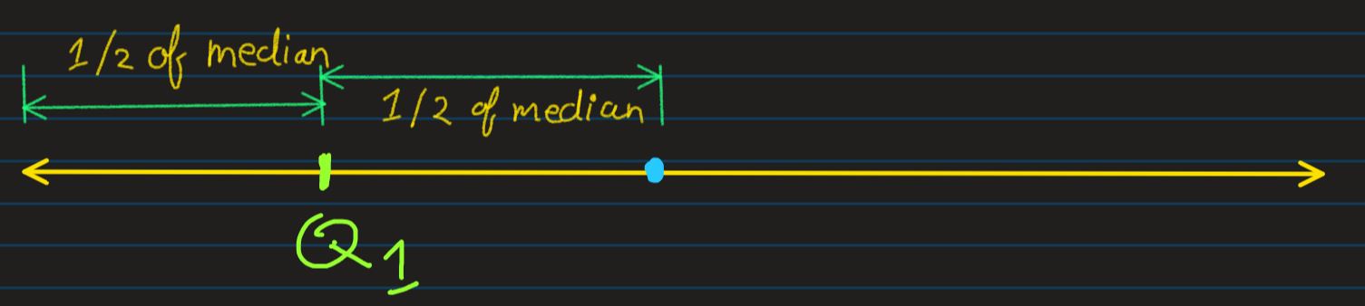
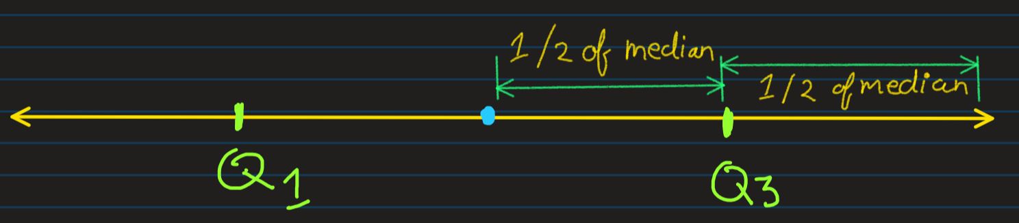
The name Q1,Q3 denotes the 1st and 3rd Quartiles and it is used to calcualte IQR
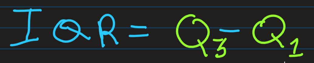
Inter Quartile Range (IQR): The differnce between Q3 and Q1 is called as Inter Quartile
Range, which is used to make Box-Whiker plots
Box-Whisker Plot:
- We can draw a box whose boundaries are Q1 & Q3
- Then we can add whiskers to the box, which would be at a distance of 1.5IQR from both the ends of the box boundary
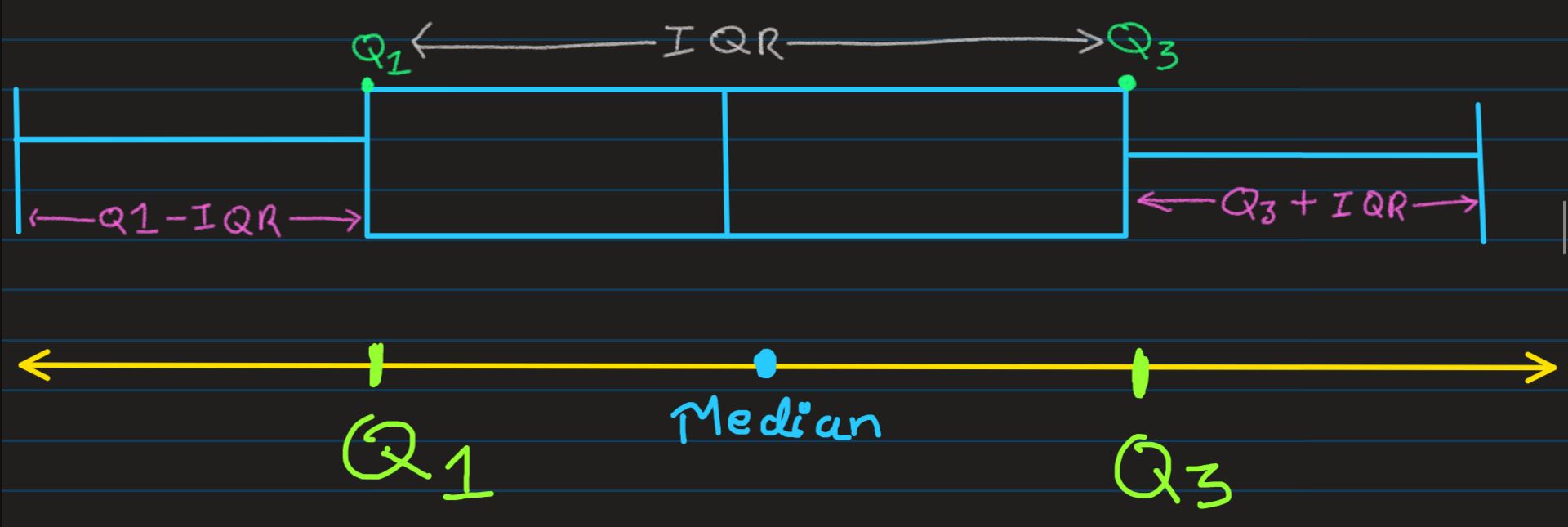 Any data point lying beyond Whiskers could be declared as Outliers
Dispersoin From Mean: Another useful way of computing the spread of data is, employing
Mean to our
rescue
Lets assume a distribution X which carries 5 observations. We can calcualte its mean
easily, and
thhus can also calcualte the deviation of each observation from the mean also very easily
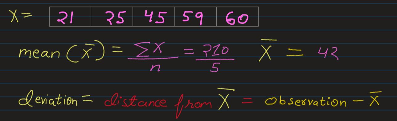
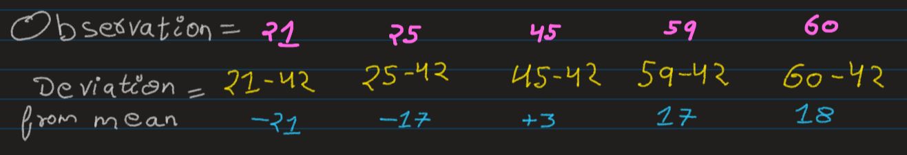
Since, the Deviation is a ditance calculation between an observation and the mean of the
distribution it
bleongs to, it can be sometimes negative in nature. This would affect the arithmetic mean.
- To resolve the problem, we can take square of each deviations, and totally get rid of negative
value
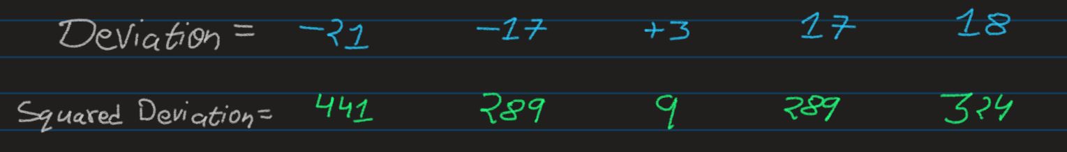
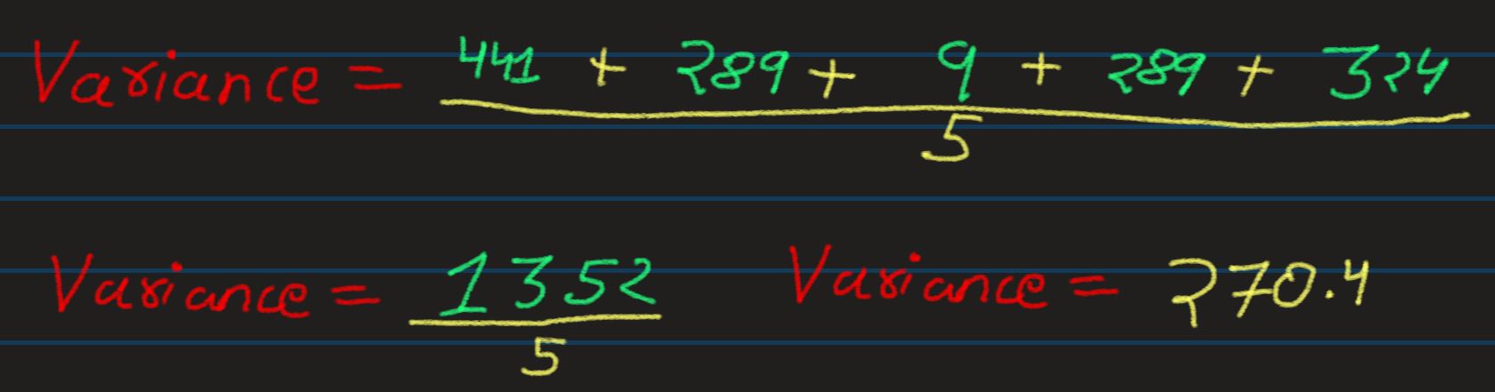
Variance: And the arithmetic mean of the Square Deviation is called Variance
 - Although Variance has a lot of merit on it own, it is still confusing for interpretation. As
we took the
square of deviations, to get rid of negative distances, the unit of the deviations, i.e.
number of
cookies sold, becomes number of cookies sold squared
- Although Variance has a lot of merit on it own, it is still confusing for interpretation. As
we took the
square of deviations, to get rid of negative distances, the unit of the deviations, i.e.
number of
cookies sold, becomes number of cookies sold squared
- To get rid of this uncomfortable cookie monster, we can apply square root to the values, and
convert
number of cookies sold squared back to number of cookies sold
- Thus, if the variance of cookies sold was 270.4 sold squared, after square root it will
become
16.443 sold
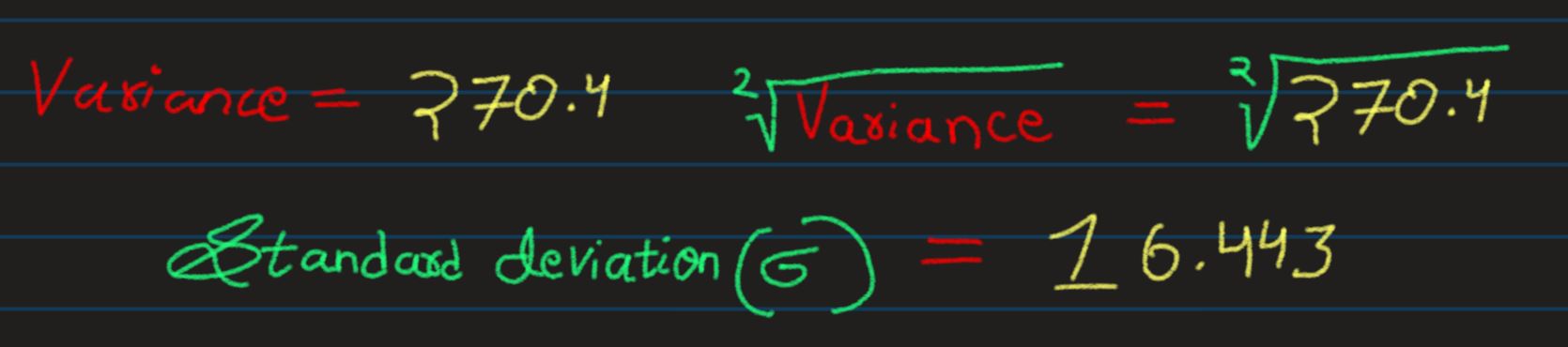
And, as you noticed, the very same square root of Variance, is also known as Standard
Deviation.
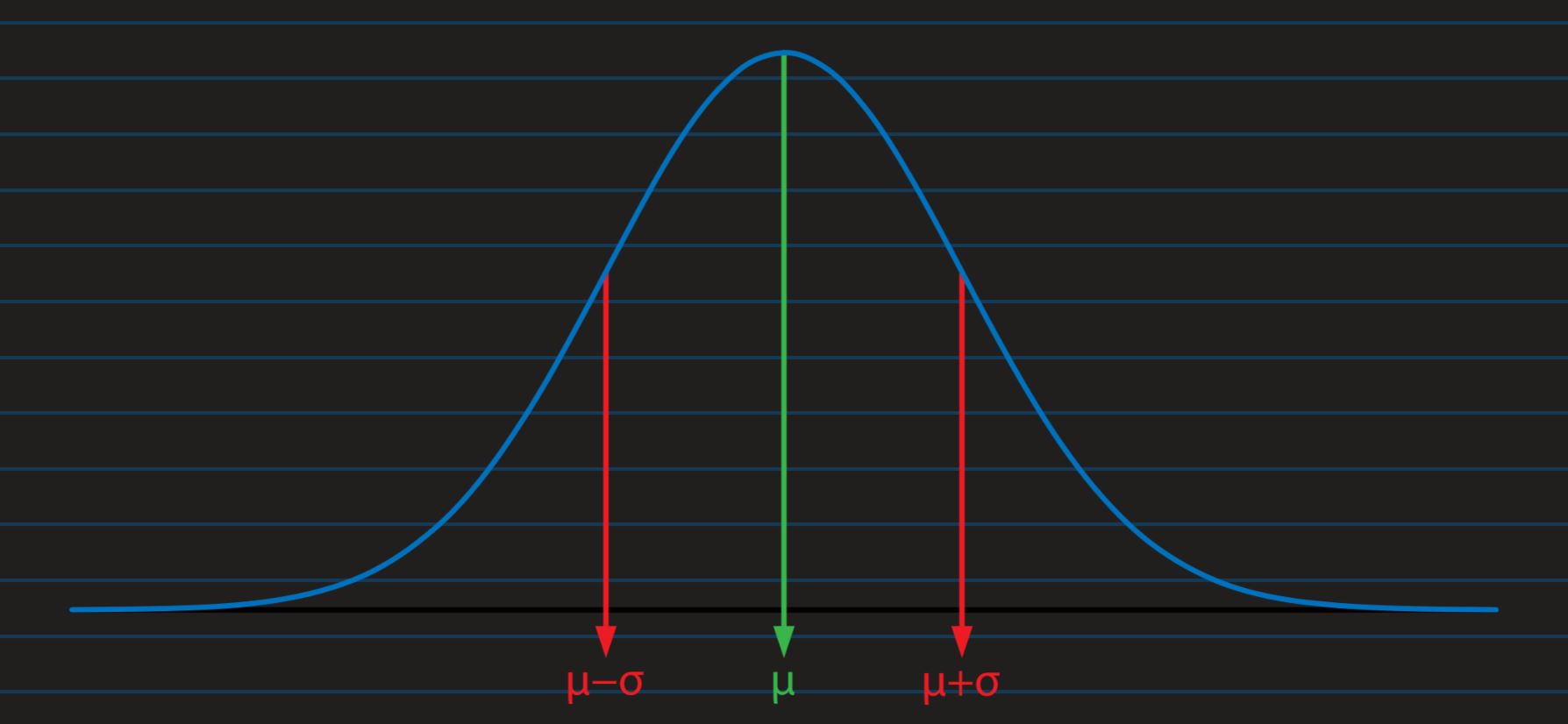
It is often useful to know how many Standard Deviation an observation is from mean, as Standard
Deviation
slices the distribution into standrd sized slices, each slice containing known percentage of
observation
And for a perfect normal distribution, approximately 68% of data is within 1 Standard Deviation,
away from
the mean(approximately two-third of data), and 95% of data is 2 Standard Deviation from
the mean
value
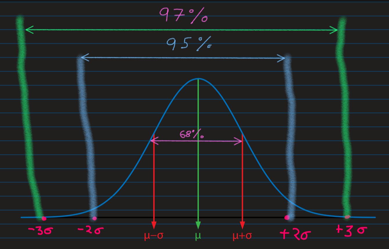 And when we say an observation "A" is 2 Standard Deviation above mean value, it means the
observation has a
Z-Score value = +2, i.e. Z-Score tells us, an observation is how much Standard
Deviation away
from the mean.
And when we say an observation "A" is 2 Standard Deviation above mean value, it means the
observation has a
Z-Score value = +2, i.e. Z-Score tells us, an observation is how much Standard
Deviation away
from the mean.
**Z-Score is usable only in case where observations exhibit normal distribution
But, what the fliffity fluffity-fluff is Normal Distribution, which I very smoothly
mentioned without
giving any context, you may ask. "Well, goood observation", I will reply.
We already know what is distribution. Lets look at what is normal and what is not normal.
Shape of Distribution
We have already seen what a Histogram looks like
In a Histogram, if we split up all the bars into infinite numbers of smaller & smaller bars,
ultimately we would end up with a smooth (continous) curved line, called as Curve of
Distribution.
Below provided video gives a nice vsual interpretation of what we just learnt
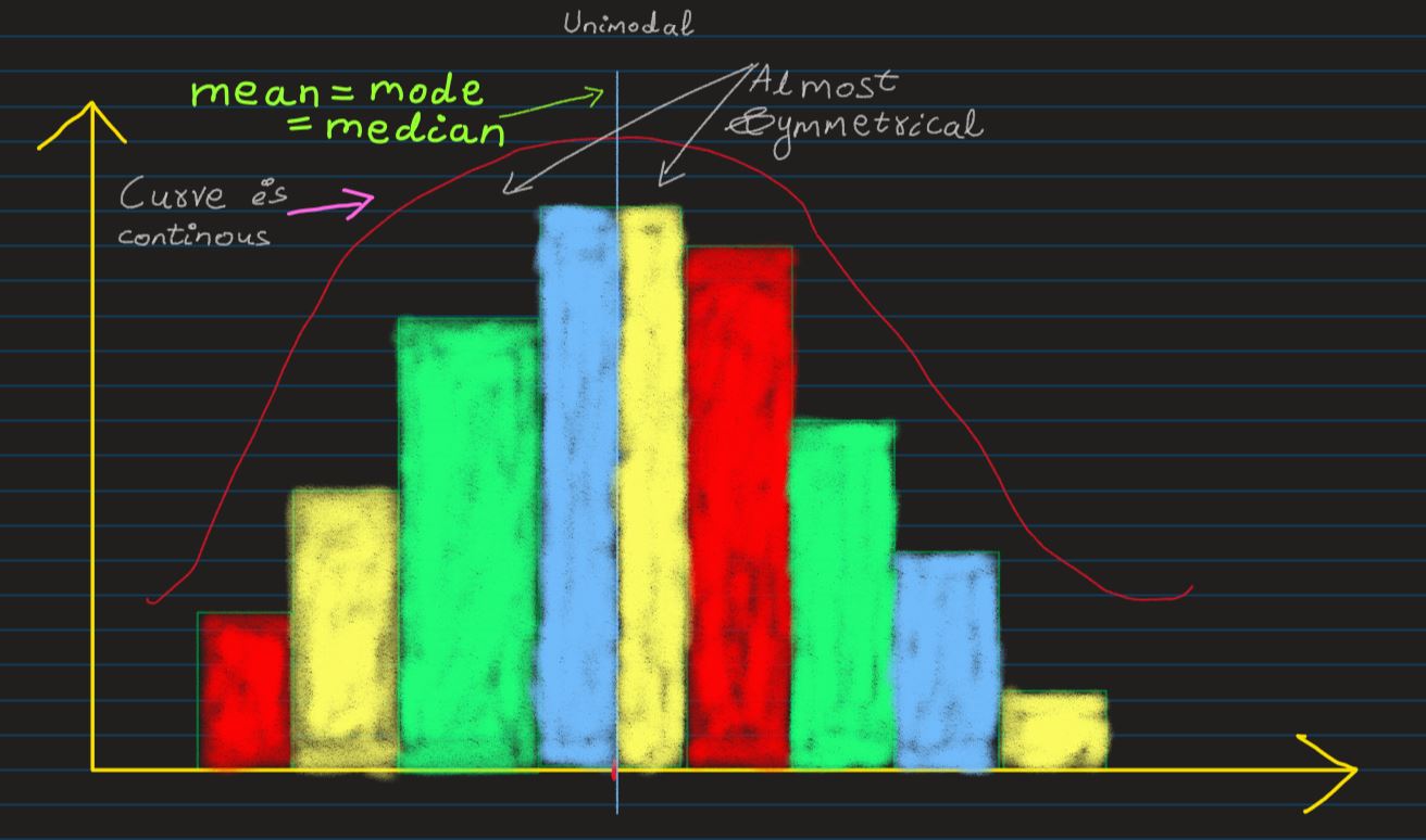
Normal Distribution: The distribution shown below is very close approximation of a
Normal/Gaussian
Distribution. For a distribution to be called as Normal, it has to have following traits:
- Unimodal, i.e. its distribution curve has only 1 peak
- symmetric bell shape, i.e. red blanket like curve over the distribution
- mean, median and mode are equal, i.e. all located at the center of the distribution
A true normal ditribution looks like this
%3Amax_bytes(150000)%3Astrip_icc()%2Fdotdash_Final_The_Normal_Distribution_Table_Explained_Jan_2020-03-a2be281ebc644022bc14327364532aed.jpg&f=1&nofb=1)
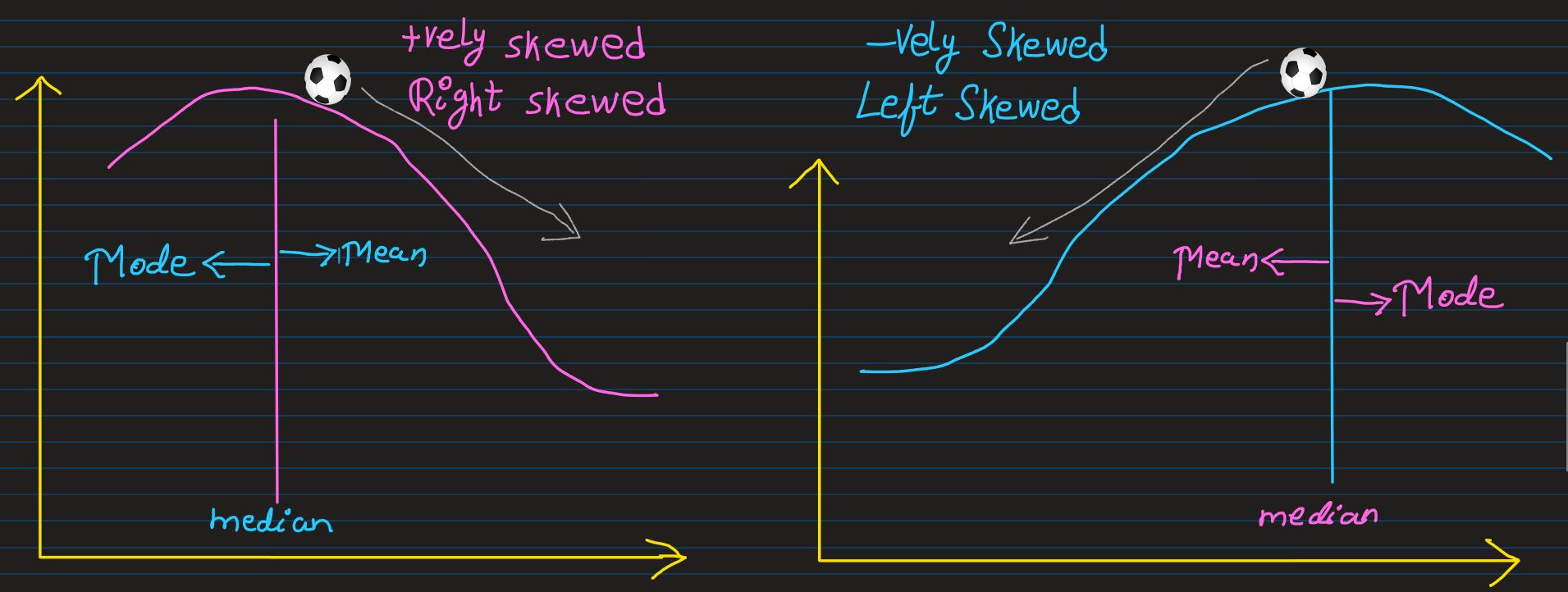
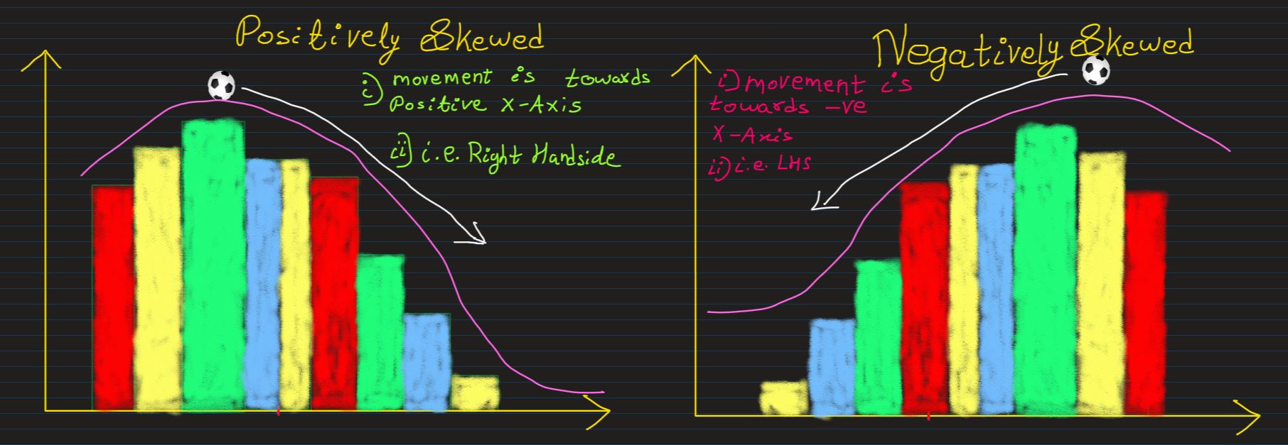
Skew: Remebering whether the curve is Right-SKewed or Left SKewed, other wise
Postively-Skewed or Negatively-Skewed has always been confusing for me
One helpful trick that I came up with to better remember it is, 'Queue' is a french word for
tail. And S(Queue) also looks
like tail. Coincidence? I don't think so!
So,
- If the tail is moving in positive direction of X-Axis, it's a Positively-Skewed
distribution
- If the tail is moving in negative direction of X-Axis, it's a Negatively-Skewed
distribution
If the skewness of a distribution is known, thier central tendency can also be estimated
- Mean is towards the direction of the slope
- Mode is towards opoosite direction of the slope