Chapters
Mathematics For Machine Learning

Probability
Chapters
Introduction
One of the primary objkective of analytics is to measure the uncertainity associated with an
event or key performance indicatorr. Axioms of probability and the concept of random variable
are fundamental bulding blocks for analytics that are used for measuring uncertainity associated
with the key performance indicators of importance of a business. Probability theory is the
foundation on which descriptive and predictive analytics models are built.
~ Credits: Business
Analytics: U Dinesh Kumar
1. Basics of Probability
Probability is a metric for determining the likelihood of an event occurring, in terms of percentage. Many things are impossible to predict with 100% certainty. One can only predict the probability of such events occurring, i.e., how likely it is to occur.
- Random Experiment: Random Experiment is an experiment in which, the ouctome is not known with certainty. Predictive Analytics mainly deals with random experiment, where the outcome is not known, with certainity, e.g. attirition rate, customer churn, demand forecasting, etc.
-
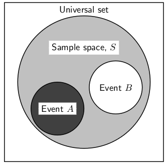
Sampel Space: Sample space is the universal set that consists of all possible
outcomes of an
experiment, represented by letter 'S', and
individual outcomes are called as 'elementary events'.
E.g. Outcome of a football match: S = {Win, Draw, Lose}
Customer Churn: s = {Churn, Won't Churn}
Life of a turbine balde in an aircraft engine: S = {X | X∈R, 0<=X<∞} -
Event: Event is the subset of sample space, and probability is calculate w.r.t. an
event
 Credits: Jobilize.com
 -
Probability Estimation: Probability of an event A, P(A), is given by:
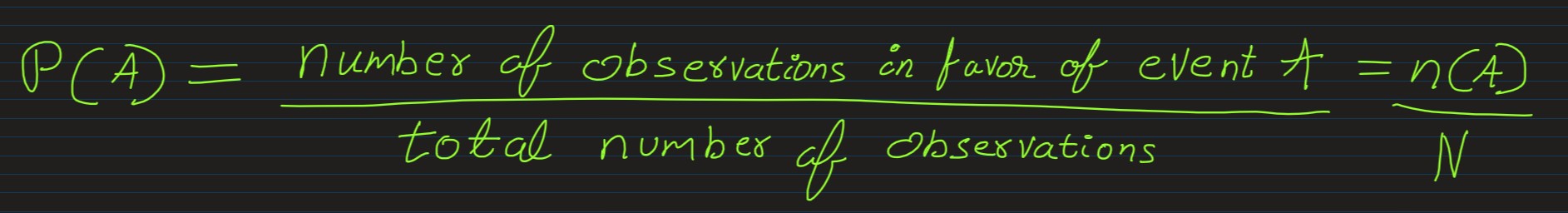
E.g. in an organization of 1000 employees, if every year 200 employess leave their job, then the probability of attririon of an employee per annum is 200/1000 = 0.2
* If the probability for an event to happen is p and the probability for it to fail is q, then p + q = 1 -
Algebra of Events: For multiple events from a sample space, we can apply and use
following algebric
expressions, to either directly achieve
or to derive results:
-
Addition Rule: The probability that events A or B will occur is given by
P(A ∪ B) = P(A) + P(B) – P(A ∩ B)
P(A or B) = P(A) + P(B) – P(A and B)
If A, B and C are mutually exclusive events, then P(A or B or C) = P(A) + P(B) + P(C) -
Multiplication Rule: The probability that two events A and B will occur in
sequence is
P(A∩B) = P(A) × P(B/A) = P(B) × P(A/B)
P(A and B) = P(A) × P(B/A) = P(B) × P(A/B)
If A, B and C are independent events, then
P(A and B and C) = P(A) × P(B) × P(C) -
Commulative Rule:
A ∪ B = B ∪ A, and A ∩ B = B ∩ A -
Associative Rule:
(A ∪ B) ∪ C = A ∪ (B ∪ C), and
(A ∩ B) ∪ C = A ∩ (B ∩ C) -
Distributive Rule:
A ∪ (B ∩ C) = (A ∪ B) ∩ (A ∪ C), and
A ∩ (B ∪ C) = (A ∩ B) ∪ (A ∩ C)
-
Addition Rule: The probability that events A or B will occur is given by
2. Axioms of Probability
- Probability of an event always lies between 0 & 1
- Probability of the universal set S is always 1
-
For any event A(e.g. probability of observing a fraudlent transaction), probability of the
complementary
event(e.g. probability of
observing a non-fraudlent transaction), written as A C is given by:
P(Ac) = 1 - P(A) -
The probability that either event A or B occurs, or both occurs, is given by
P(A ∪ B) = P(A) + P(B) - P(A ∩ B) -
Marginal Probability: Marginal Probability is simply a probability of an event X,
denoted by P(X),
without any conditions
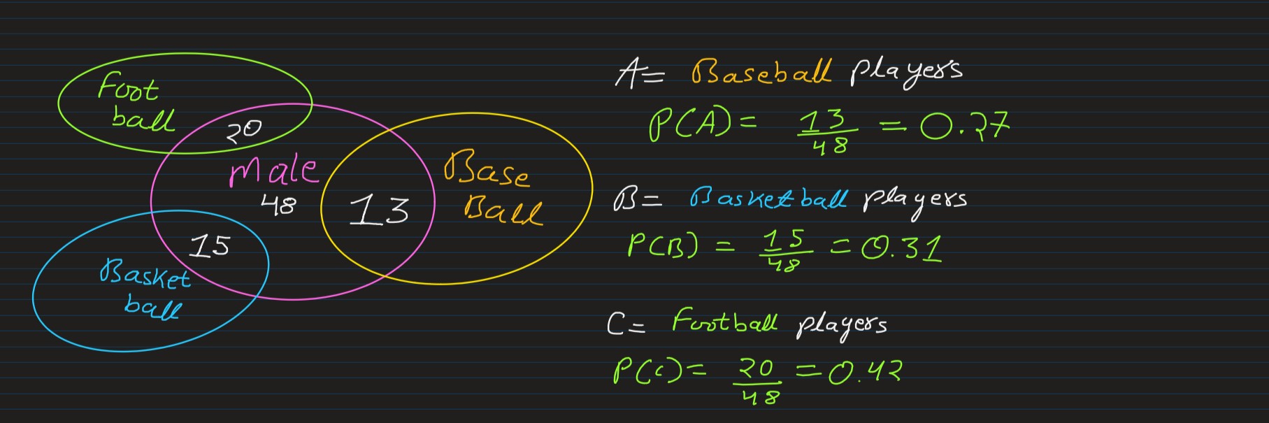
-
Joint Probability: Joint probability is the likelihood that two events will happen at
the same
time. It's the probability that event X occurs at the same time as event Y.

Conditions being:- events A and B must happen at the same time
- events A and B must be independent (non-interfering) of each other

The word joint comes from the fact that we’re interested in the probability of two things happening at once, like here, male & baseball
So, according to our above statd Joint Probability forumula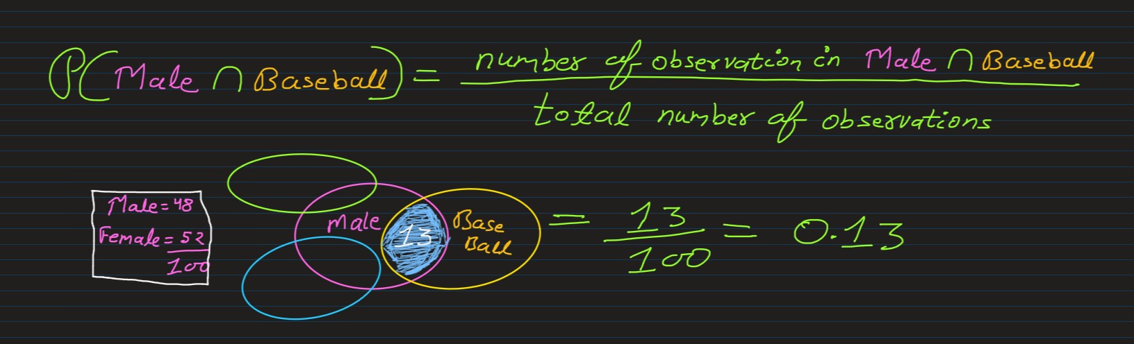
-
Conditional Probability is known as the possibility of an event or outcome happening,
based on the
existence of a previous event or outcome
If events A & B are events in a sample space, then the conditional probability of the event B, given that the event A has already happened, is denoted by P(B|A), and is defined as: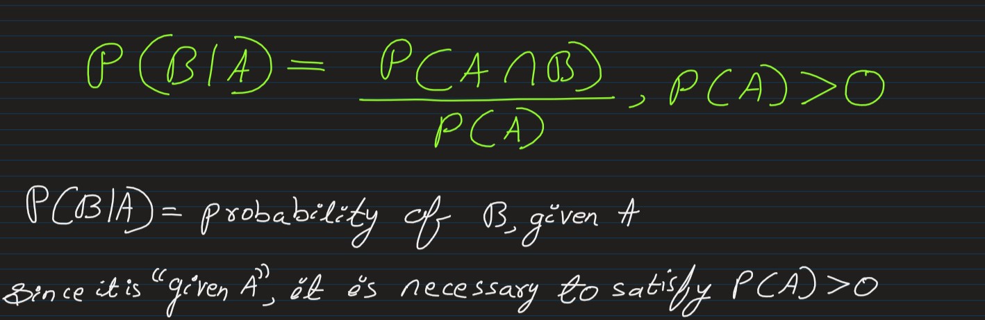
For example, we might expect the probability that it will rain tomorrow (in general) to be smaller than the probability it will rain tomorrow given that it is cloudy today. This latter probability is a conditional probability, since it accounts for relevant information that we possess.
Mathematically, computing a conditional probability amounts to shrinking our sample space to a particular event. So in our rain example, instead of looking at how often it rains on any day in general, we "pretend" that our sample space consists of only those days for which the previous day was cloudy.
3. Application of Probability
Association Rule Learning: Market Basket Analysis is used frequently by retailers, to
predict items
frequenlty bought together
by the customers, to improve thier product promotions. And, Association Rule Learning is a
method of finding
associations between different entities.
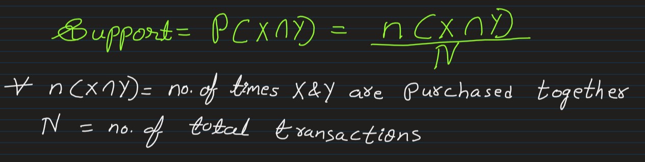
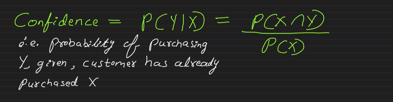
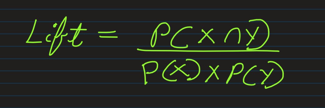
And the Strength-of-Association between 2 items can be measured using Support, Confidence & Lift
-
Support:
-
Confidence:
-
Lift:
4. Bayes Theorem
Bayes Theorem can be understood as the description of the probability of any event which
is
obtained by prior knowledge about the event
We can say that Bayes’ theorem can be used to describe the conditional probability of any event
where we
have
- data about the event
- prior information about the event
- with the prior knowledge about the conditions related to the event
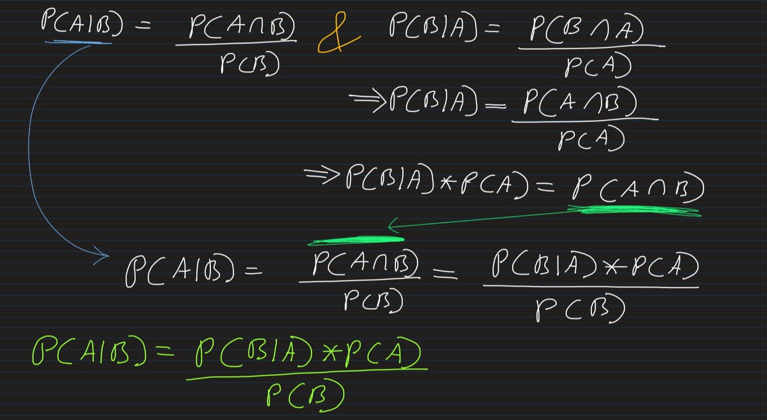
As per Conditional Probability, we know that
-
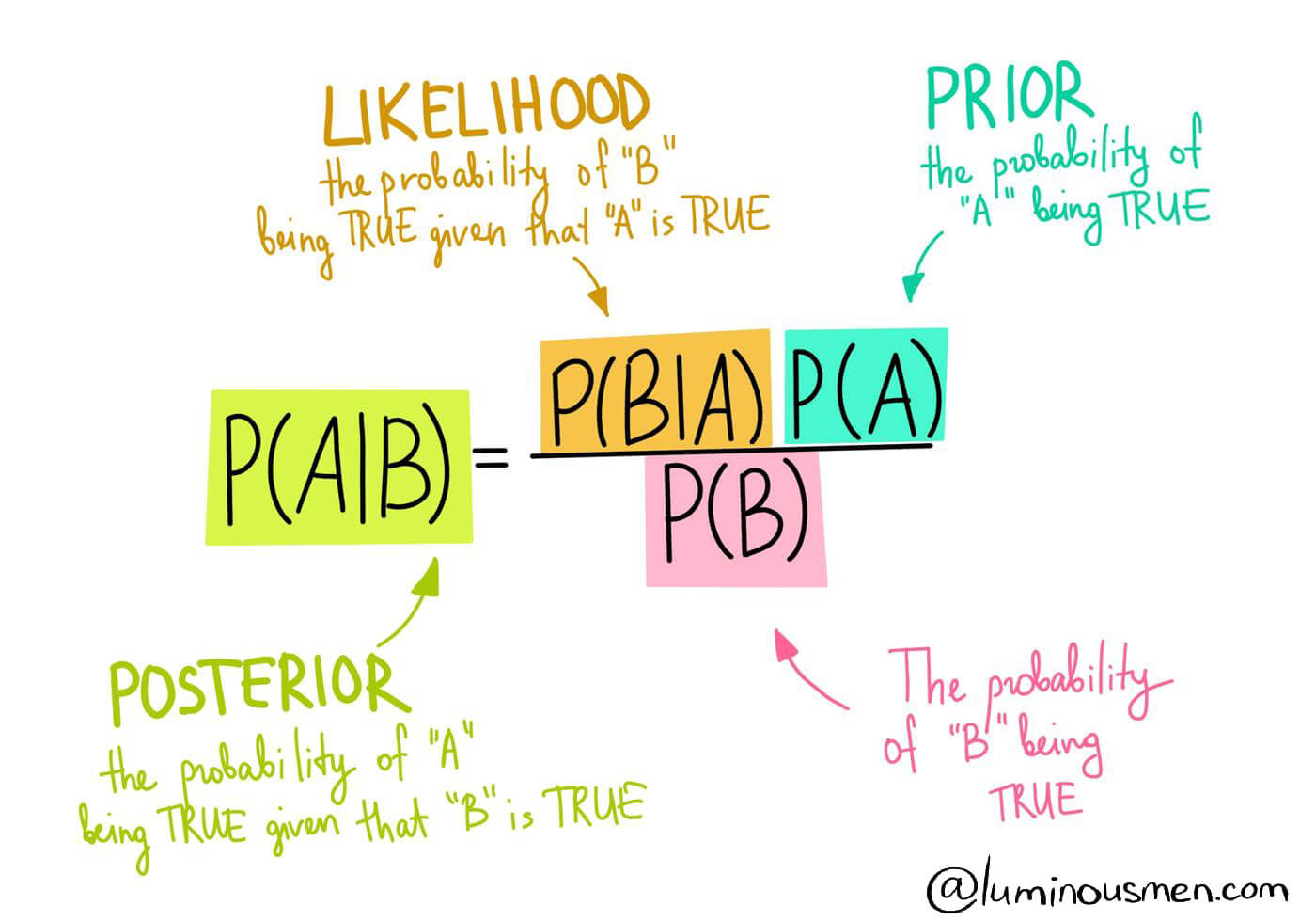
Prior Probability:
In the formula of the Bayes theorem, P(A) is the Prior Probability
According to Bayesian statistical inference we can define the Prior Probability or Prior, of an uncertain quantity as the probability distribution that would express one's beliefs about this quantity before some evidence is taken into account
For example, the relative proportions of voters, who will vote for a particular politician in a future election
P(A) expresses one’s belief of occurrence of A before any evidence is taken into account -
Likelihood Function:
P(B|A) is the likelihood function which can be simply called the likelihood
It can be defined as the probability of B when it is known that A is true
Numerically it is the support value where the support to proposition A is given by evidence B - Posterior Probability: P(A|B) is the posterior probability or the probability of A to occur given event B already occurred
A great article on Monty Hall Problem, which is solved using Bayes Theorem. Go through it once before proceeding further about Random Variables and Distribution Functions
Relationship Between Conditional Probability and Bayes Theorem
** The numerator, i.e. P(B|A)*P(A) says that, both the event has occured, i.e.
Event (A) &
Event (B|A)
And from the concept of Conditional Probability, the denominator P(B) says,
P(Numerator|B), i.e.
Probability of Numerator happening, give event B has already happened
Random Variable
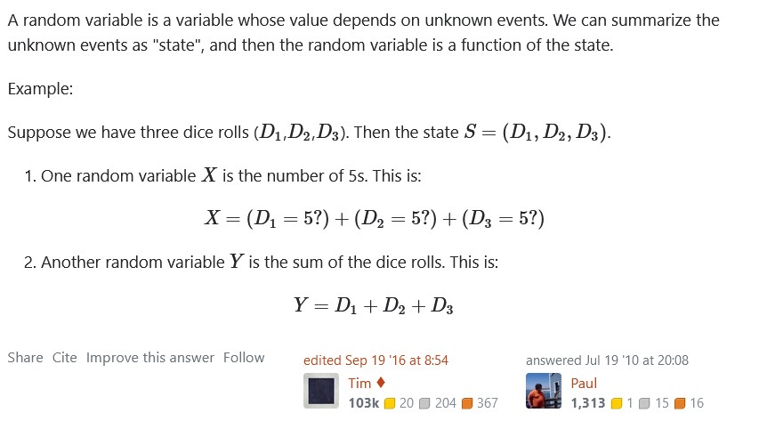
Random Variable: A random variable is a variable whose value depends on unknown
events.
We can summarize the unknown events as "state", and then the random variable is a function
of
the state
A variable is a symbol that represents some quantity, whereas, a random
variable
is a value
that follows some probability distribution.
Discrete Random Variable: If a random variable can assume only a finite, or
countably
infinite set of
values, then it is called as a Discrete Random Variable
E.g. 5 pencils, 100 vehicles, 10,000 user registraions
Continous Random Variable: If a rancom variable can take a value from an infinite
set of
values, it
is called as Continous Random Variable
E.g. length of pencil (7cm or 7.32cm or 7.321456894123cm)
Functions to consider when we have
- Discrete Random Variable: Probability Mass Function
- Continous Random Variable: Probability Density Function
- Both cases: Cumulative Distribution Function
The term probability relates is to an event and probability distribution relates is to a random variable.
A great video about probability distribution:
It is a convention that the term probability mass function refers to the probability function of a discrete random variable and the term probability density function refers to the probability function of a continuous random variable
- PMF: When the random variable is discrete, probability distribution means, how
the total probability is distributed over various possible values of the random variable
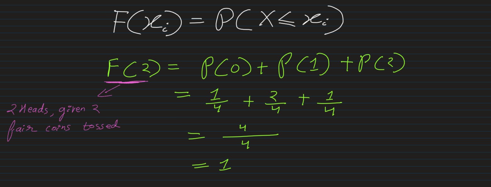
Consider the experiment of tossing two unbiased coins simultaneously. Then, sample space S associated with this experiment is:
S = {HH, HT, TH, TT}
If we define a random variable X as: the number of heads on this sample space S, then
X(HH) = 2, X(HT) = X(TH)=1, X(TT) = 0
The probability distribution of X is then given by P(x) = x/n
P(2) = 1/4; P(1) = 2/4; P(0) = 1/4
Which could be represented as in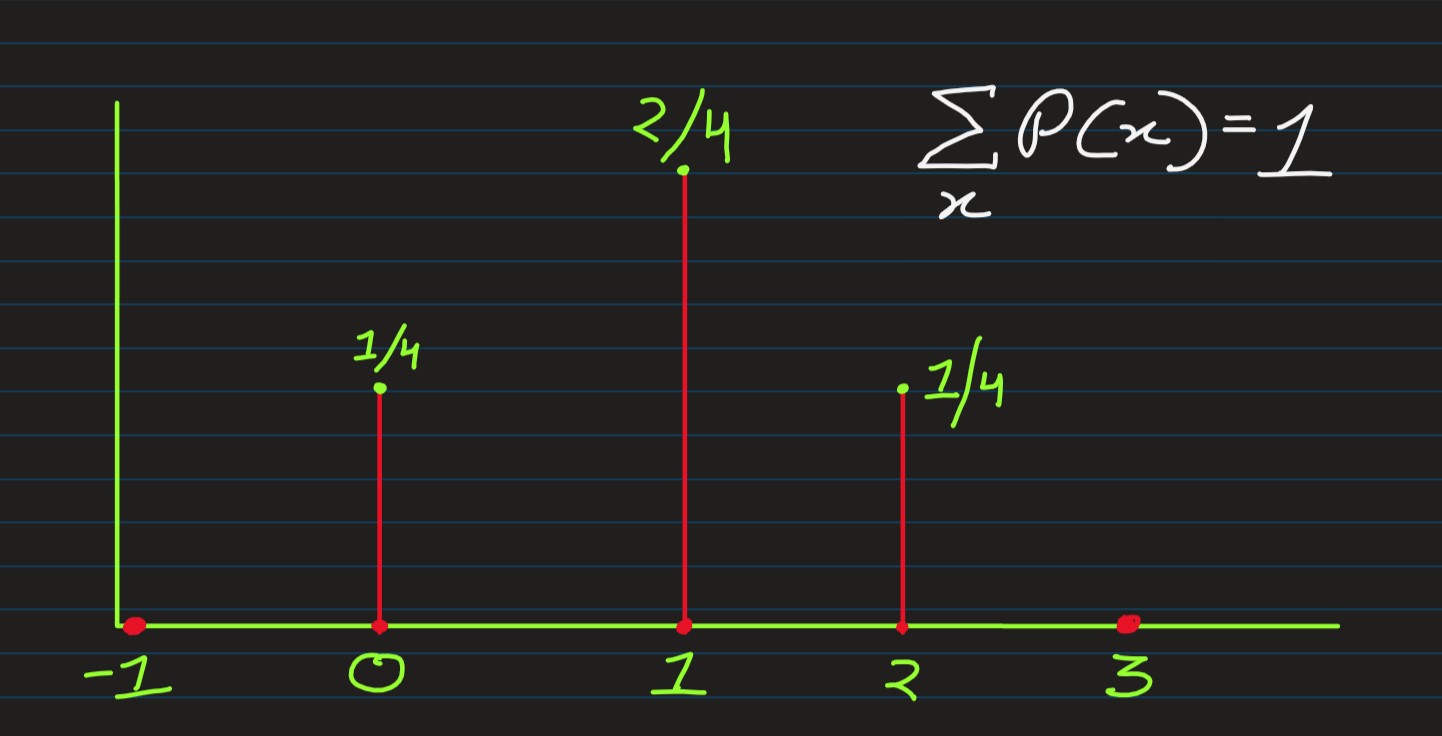
For a discrete random variable, we consider events of the type {X=x} and compute probabilities of such events to describe the distribution of the random variable. This probability, P{X=x}=p(x) is called the probability mass function -
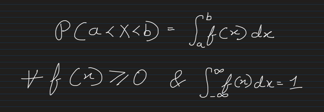
PDF: A continuous random variable is described by considering probabilities for
events of the
type (a<X<b).
The probability function of a continuous random variable is usually denoted by f(x) and
is called a
probability density function
It is a function whose value at any given sample (or point) in the sample space (the set of possible values taken by the random variable) can be interpreted as providing a relative likelihood that the value of the random variable would be close to that sample. Credits: Wikipedia.com
 -
CDF: Cumulative Distribution Function, F(Xi), is the probability that the random
variable X takes
values less than or equal
to Xi, i.e.
Distributions
The distribution is simply, the assignment of probabilities, to sets of possible values of the random variable. And, a probability distribution is a statistical function, that describes all the possible values and likelihoods that a random variable can take within a given range
-
Bernoulli Distribution: Any event, which has 1 trial with 2 possible events,
follows Bernoulli
Distribution, e.g. Coin Flip
 Credits: Wikipedia
-
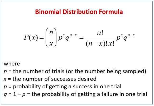
Binomial Distribution: Binomial Distribution helps in getting number of times we
expect to get a
specific outcome. As,
its graph represents our likelihood of attaining our desired outcome, a specific number
of times
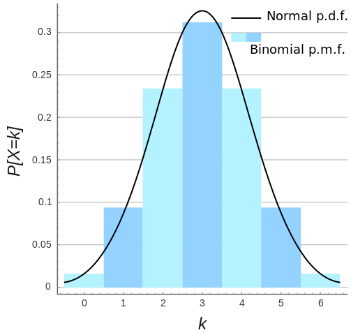 Binomial probability mass function and normal probability density function approximation for n = 6 and p = 0.5
Credits: Wikipedia
In order for a random variable to be considered for Binomial Distribution, it needs to satisfy following conditions:
- Only 2 unique outomes possible, i.e. Bernoulli Trials
- Objective: probability of getting k successes, out of n trials
- Each trial is a "yes-no asking" independent event
- Probability P is constant, and doesn't varies between trials (probability of getting tails doesn't changes after some n-p trials)
 Few good examples include binary classifications like churn and wont churn, fraud
transaction & non-fraud transactions, loan emi default and no default, etc
Few good examples include binary classifications like churn and wont churn, fraud
transaction & non-fraud transactions, loan emi default and no default, etc
-
Poisson Distribution: Sometimes we are interested in the count of events, e.g.
number of orders
in an ecommerce website, number of cancelled orders,
number of customer complaints in a telecom company, etc. In such cases, we need
probaility distribution
of number of events, i.e. Poisson Distribution.
 Credits: Wikipedia
E.g. the number of mails you receive monthly, are countable and independent of each other.
It is a poisson distribution event, as it deals with the frequency at which an event occurs in a specific interval, instead of the probability of the event, it wants to know how often an event occurs, for a period of time
Another example, firefly lighting up 3 times in 10seconds -
Geometric Distribution: Sometimes, we're more interested to discover about the
number of failures
between 2 success in Bernoulli Distribution, e.g. as
in case of duration between 2 purchse of visit to the store. Here, if each day is 1
trial, and the
outcome is purchased & not-purchsaed, then each point in
x-axis of the bernouli graph would be a unique single day, which could be either
purchased or
not-purchsaed. And Geometric Distribution will help us in knowing
what is the duration between 2 purchases
I.e. Geometric Distribution si the number of Bernoulli Trials required to achieve success. It represents a random experiment in which the random variable predicts the number of failures before the success.
A great explanation of Geometric Distribution: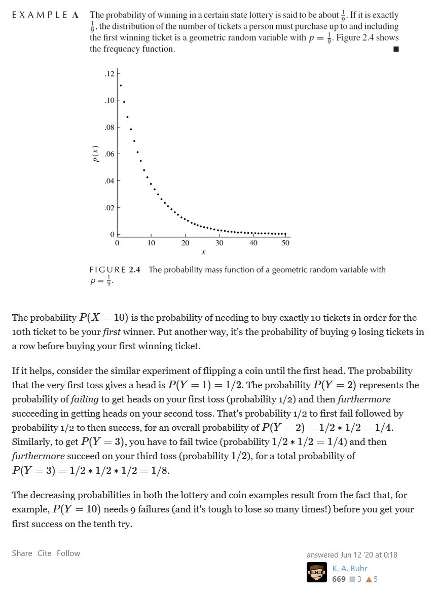 Credits: K. A. Buhr
- Continous Distribution:
-
Uniform Distribution: In statistics, uniform distribution refers to a type of
probability
distribution in which all outcomes are equally
likely. E.g. A deck of cards has within it uniform distributions because the likelihood
of drawing a
heart, a club, a diamond, or a spade is
equally likely. A coin also has a uniform distribution because the probability of
getting either heads
or tails in a coin toss is the same.
There are two types of uniform distributions: discrete and continuous. The possible results of rolling a die provide an example of a discrete uniform distribution : it is possible to roll a 1, 2, 3, 4, 5, or 6, but it is not possible to roll a 2.3, 4.7, or 5.5. Therefore, the roll of a die generates a discrete distribution with p = 1/6 for each outcome. There are only 6 possible values to return and nothing in between[1].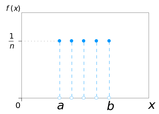 Credits: Wikipedia
Some uniform distributions are continuous rather than discrete. An idealized random number generator would be considered a continuous uniform distribution . With this type of distribution, every point in the continuous range between 0.0 and 1.0 has an equal opportunity of appearing, yet there is an infinite number of points between 0.0 and 1.0[2].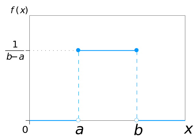 Credits: Wikipedia
-
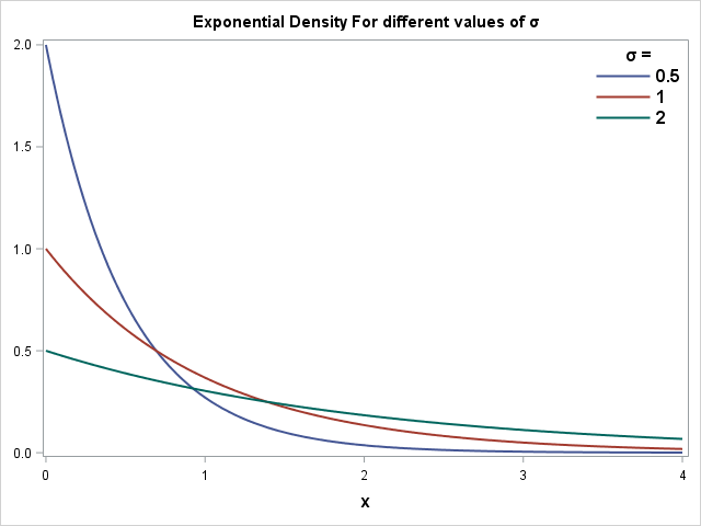
Exponential Distribution: In Exponential Distribution, the events occur
continuously and
independently at a constant average rate.
The exponential distribution, Erlang distribution, and chi-square distribution are
special cases of the
gamma distribution
 Credits: Sasnrd.com
-
Normal Distribution: Normal distribution, also known as the Gaussian
distribution, is a
probability distribution that is symmetric about the mean, showing that data near the
mean are more
frequent in occurrence than data far from the mean. In graph form, normal distribution
will appear as a
bell curve[3].
:max_bytes(150000):strip_icc()/dotdash_Final_The_Normal_Distribution_Table_Explained_Jan_2020-03-a2be281ebc644022bc14327364532aed.jpg) Credits: Investopedia.com
Credits: Investopedia.com
A normal random variable with mean = 0 & standard deviation = 1 is called as Standard Normal Variable, and usually represented by Z
-
Chi-Squared Distribution: When k independent standard normal random variable are
squared and
summed together, the non-parametric distribution
obtained is called as Chi-Square Distribution with K-Degrees of Freedom.
Used to check the relationships between categorical variables, to study the sample variance where the underlying distribution is normal, and most importantly, to conduct a The chi-square test (a goodness of fit test) -
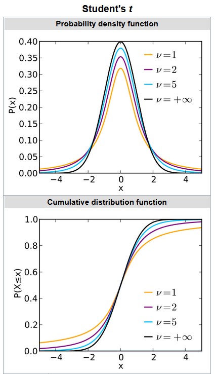
Student's t-Distribution: The distribution arise when estimating the mean of a
normally
distributed population in situations where the sample size is small and the population's
standard
deviation is unknown
-
F-Distribution: is a continuous probability distribution that arises frequently
as the null
distribution of a test statistic, most notably in the analysis of variance (ANOVA) and
other F-tests.
Null Distribution is the probability distribution of the test statistic when the null hypothesis is true
Books
- Math 201: Linear Algebra by Jacob Bernstein
- Mathematics for Machine Learning authored by Marc Peter Deisenroth
- Linear Algebra and Optimization for Machine Learning authored by Charu Aggarwal